One variable Linear regression using R

In this post we will start talking about modeling and nothing better and easier than Linear Regression. For a better understanding of Linear Regression concepts, please visit this site.

Before we start our modeling we need to load the dataset into R. I would be using RStudio for creating this model.

Loading Data: The dataset is loaded using the read.csv functions. there are other options as well to load data but since the data we would be working with is in the csv (Comma Separated Values) format, we are using this command. The typical syntax is

Data1 = read.csv(“dataset_name.csv”)

Structure of the data: Before we work on the data, we need to look at the contents of the dataset namely the number of data points, the names of the variables and their few values, a few statistics about the data. In R, there are 2 commands which can be used (str and summary)

str(Data1)

In the image below you will see that the dataset has 25 observations and 7 variables. The names and the initial values of all the variables are also listed

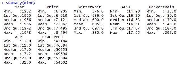
summary(Data1)

In the image below you will see that the summary function lists a few statistics for the different variables. Statistics include Minimum, maximum, 1^st and 3^rd quartiles, the mean and the median

After getting to know about our dataset we will start creating the model. The syntax is:

Model1 = lm(DV ∼ IV, data = dataset name)

• lm is the R function to create linear regression models
• DV is the dependent variable
• The ~(tilde) sign in between the DV and the IV tells R to create a linear model between the DV and IV
• IV is the Independent variable
• data = dataset name helps R identfiy the dataset that it will be working on to create the model

The syntax above would result in creating a Linear regression of the form:

 

 

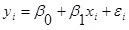
The syntax mentioned above would create the model but nothing would be displayed in the console window. To see the results of the linear model, we would need to look at the summary of the model using:

summary(Model1)

There are various things that we can see in the summary of the model as shown in the image below. We will look at the individual elements in the next few sections

 

Call: The first thing we see specifies the code used to create the linear regression model

Residuals: Gives us the a few statistics of the error terms. This can be used to calculate SSE (Sum of squared errors). The model has a vector by the name “residuals” which has values for all the error terms. Type Model1$residuals to see the values of each error term

Coefficients:

• Estimate column gives the values of the coefficient for the intercept (β0) and the independent variable (β1)
• Std. Error column gives a measure of how much the coefficient is likely to vary from the estimate value
• t-value: The t value is the estimate divided by the standard error. It will be negative if the estimate is negative, and positive if the estimate is positive.The larger the absolute value of the t statistic, the more likely the coefficient is to be significant, so we want variables with a large absolute value in this column
• Pr( > |t| ): The last column gives the probability that a coefficient is actually 0. It will be large if the absolute value of the t statistic is small, and it will be small if the absolute value of the t statistic is large. We want variables with small values in this column. This is a lot of information, but the easiest way in R to determine if a variable is significant is to look at the stars at the end of each row. Three stars is the highest level of significance, and corresponds to a probability less than 0.001. The star coding scheme is explained
  at the bottom of the coefficient output. Three stars corresponds to probability values between 0 and 0.001, or the smallest possible probabilities. Two stars is also very significant, and corresponds to a probability between 0.001 and 0.01. One star is also significant, and corresponds to a probability between 0.01 and 0.05. A period, or dot, means that the variable is almost significant, and corresponds to a probability between 0.05 and 0.1.

To the bottom of the image, we see Multiple R squared, which is the standard R squared value (For details please visit this site)

Besides Multiple R squared is the term Adjusted R squared which adjusts the R squared value to account for the number of independent variables used relative to the number of data points. Important Note: Multiple R squared always increases if we add more independent variables but Adjusted R squared could decrease if an independent variable is not helpful to the model.

Also visit R Bloggers.com for much more interesting things happening in the R community.

In the next post we will look at linear regression using multiple independent variables.. Till such time, happy modeling